Analyzing big data, or more precisely, datasets with high cardinality, comes with strenuous memory requirements.
For example, if we own a service with a billion daily users and we want to record the latency every user experiences when they access our service, in the worst case, this can result in a billion possible values, bounded only by their type, such as the float64 number space.
latency: f64This dataset (unit: milliseconds) contains numbers like:
Latency dataset
[30.92, 30.95, 41.2,...]This cardinality can be reduced with histograms. We can create buckets to group the most important categories of metrics we want to record. These categories are:
- Less than 10 milliseconds
- Greater than 10 milliseconds and less than 20 milliseconds
- Greater than 20 milliseconds.
With these categories, the numbers in our original dataset will all be recorded in the “greater than 30 milliseconds” bucket rather than in three distinct buckets. This data structure has helped us summarize our distribution. We have successfully reduced our cardinality from a billion to three.
A different kind of summary
The Q-Digest data structure, similar to a histogram, summarizes distributions but in a different way. It retains the dense parts of the distribution while compressing the sparse parts. This means it preserves important information! while staying within predictable memory constraints.
For example, if we have a dataset of all the ages of our 1 billion users, I’m using ages instead of latency because one limitation of q-digests is that it only works with unsigned integers (T-Digest supports floats).
Age dataset
[1, 1, 2, 3, 4 , 4, 4, 4, 4, 5, 5, 5, 5, 5, 6, 6, 6, 6, 6...]The numbers 4, 5, and 6 have the highest frequencies in the dataset. A q-digest can summarize this like:
| Number | Occurence |
|---|---|
| 6 | 5 |
| 5 | 5 |
| 4 | 5 |
| 1,2,3 | 4 |
The sparser elements in the dataset, numbers 1,2 and 3 have been compressed! This is why a q-digest is lossy and probabilistic. It's a lossy kind of compression because we can’t recreate the original dataset from this data structure.
With what we have, the question, “How many times did the number 1 show up in our dataset ?” can't be answered unequivocally. It can be once or twice. Same for all the other numbers that have been compressed.
A q-digest is also tunable. It allows us set a threshold for compression. For the age dataset, we can say our threshold is 5 because items with frequencies less than 5 (1,2 and 3) were compressed.
Fine-tuning and choosing the right threshold is very important because if it's too high, then we don’t compress anything, which means we gain nothing from the q-digest. If it's too low, we compress everything, which means that we get useless information from the q-digest.
For example, if everything is compressed:
| Number | Occurence. |
|---|---|
| 1,2,3,4,5,6 | 19 |
This result is useless as we can’t tell which numbers have the highest frequencies, for example.
Error tolerance
The threshold used for compression is a function of the error tolerance and the number of items in the q-digest.
For example, The age dataset has 19 items. if we set the error tolerance to 25% (0.25),
then the threshold is 19 * 0.25 = 4.75. This means every item with a frequency less than 4.75 is compressed.
Building a Q-digest
At its core, a q-digest is a binary tree. This tree comprises of all the numbers the q-digest should be aware of.
To better understand this, I wrote a Rust library called Quest that implements a q-digest.
Now, let's try to build one for the age dataset.
Quest::new(
    min, // 1
    power_of_two, // 3
    error_tolerance, // 0.25
    compress_after // 19
)
The numbers in the age dataset range from 1 to 6. This means the min argument would be 1.
The power_of_two argument will be 3 because 2^3 = 8, which is enough to cover the maximum value of the dataset, 6.
It needs to be a power of 2 because we need to build a balanced tree.
This also means that the range is bounded, and it doesn't accept arbitrary numbers, even if this can be handled gracefully 1.
error_tolerance has been explained and will stay at 25%.
Compression can be intrusive, as we’ll have to perform a post-order traversal of the entire tree to find candidates to compress. This will be expensive to do every time an item is inserted into our tree, so compress_after tells us how long to wait before we compress so we can amortize the cost.
It's not really relevant in this example, and we can set it to 19, which means compress at the end since we know our dataset has 19 items.
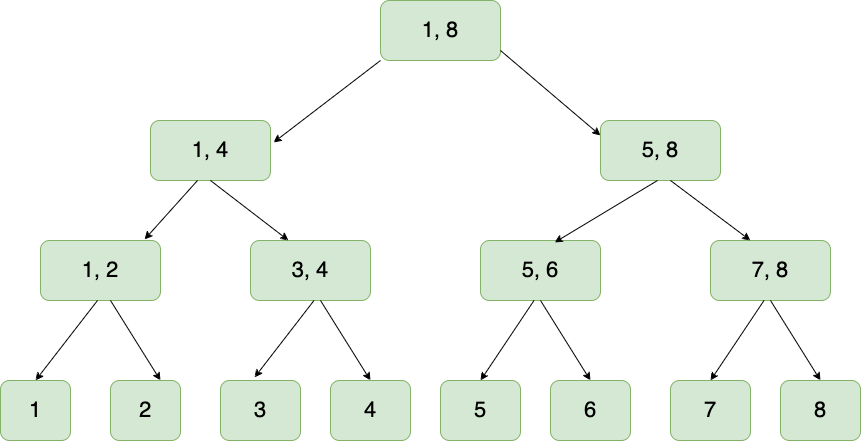
Our newly initialized tree will look something like:
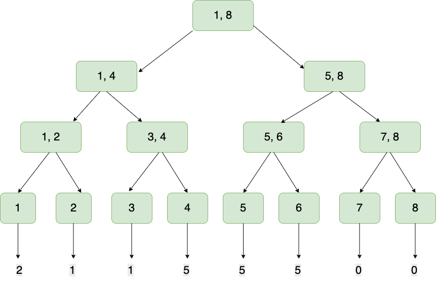
After all the items from the dataset have been inserted, the cumulative counts of each item are stored in the leaf nodes:
When the summation of frequencies in a sub-tree ie. the leaf nodes and their parent don’t meet the threshold, then they are compressed. In this case, the leftmost and rightmost subtrees have counts 3 and 0, respectively, and the threshold is 4.75:
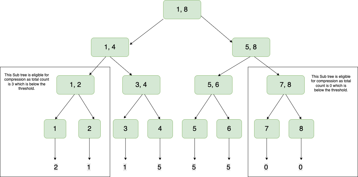
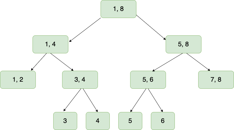
This means that the leaf nodes collapse into their parent, and we have reclaimed some memory:
Queries
This data structure allows us to perform queries like:
1. Quantile Query This answers the question "what number is at this quantile". This is achieved by doing an inorder traversal.
2. Inverse Quantile Query This is the opposite of a quantile query. It answers the question "On what quantile is this number placed". This is achieved by doing an inorder traversal.
3. Range Query This answers the question "how many numbers in this dataset are between numbers x and y". This is achieved by taking the difference of two inverse quantile queries.
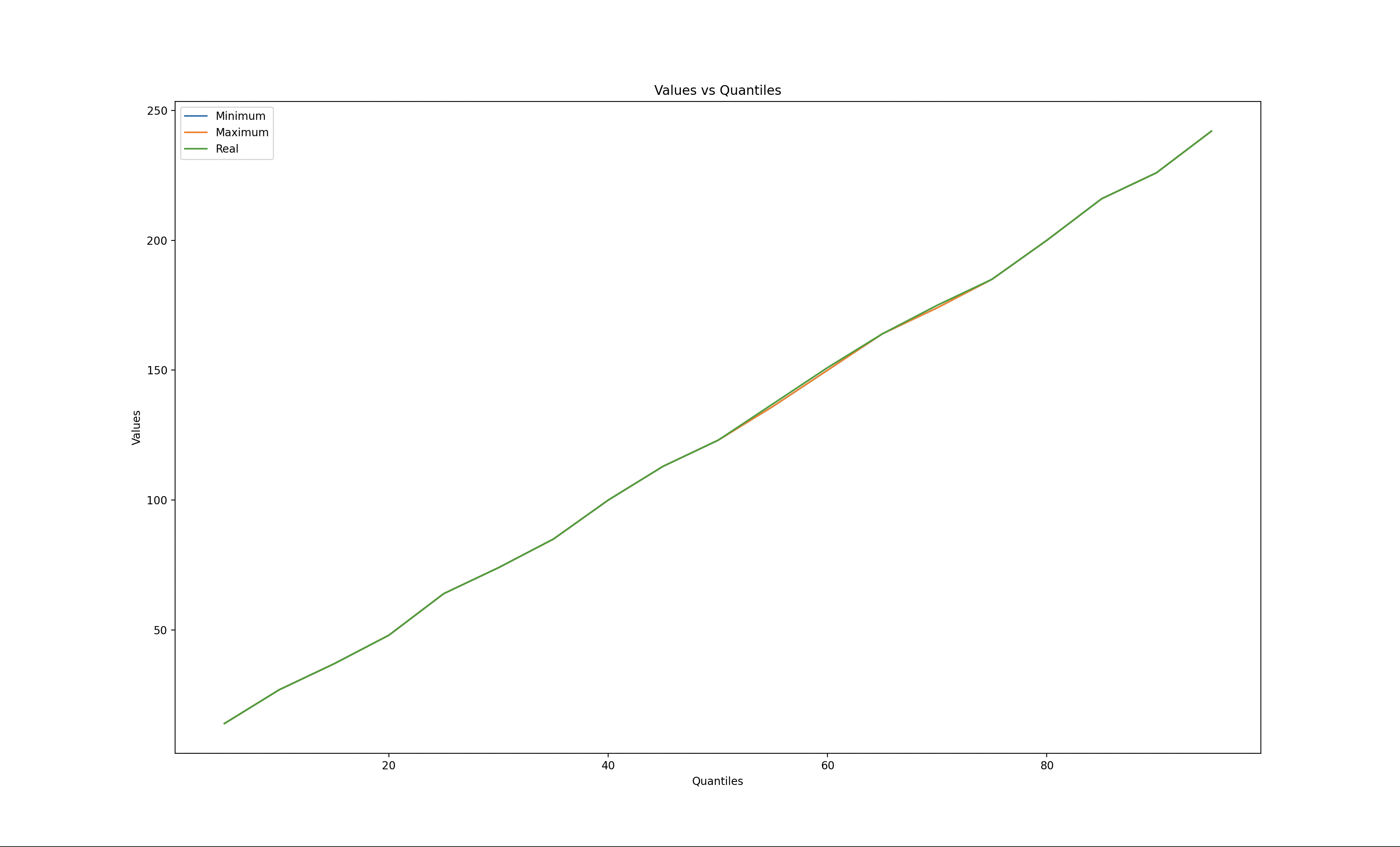
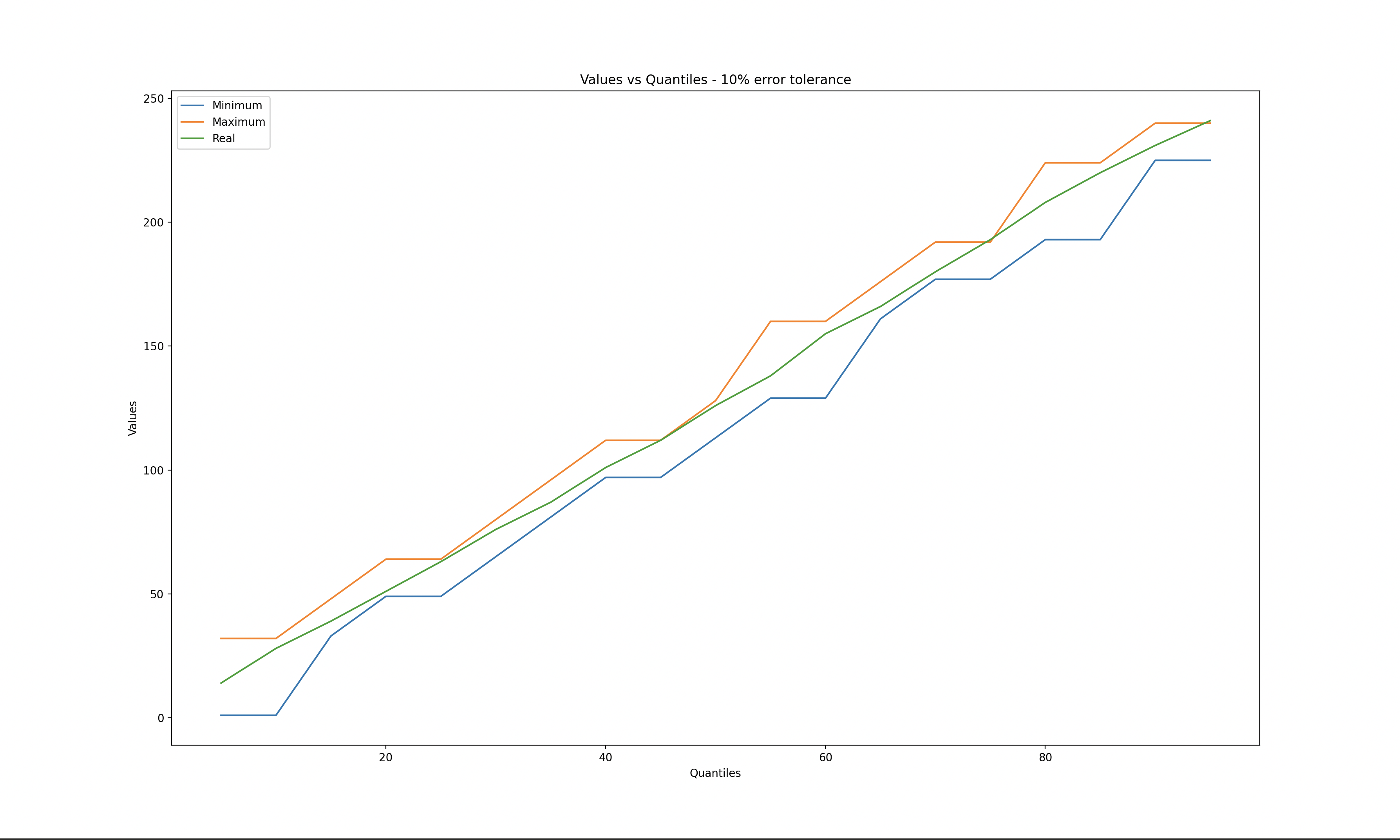
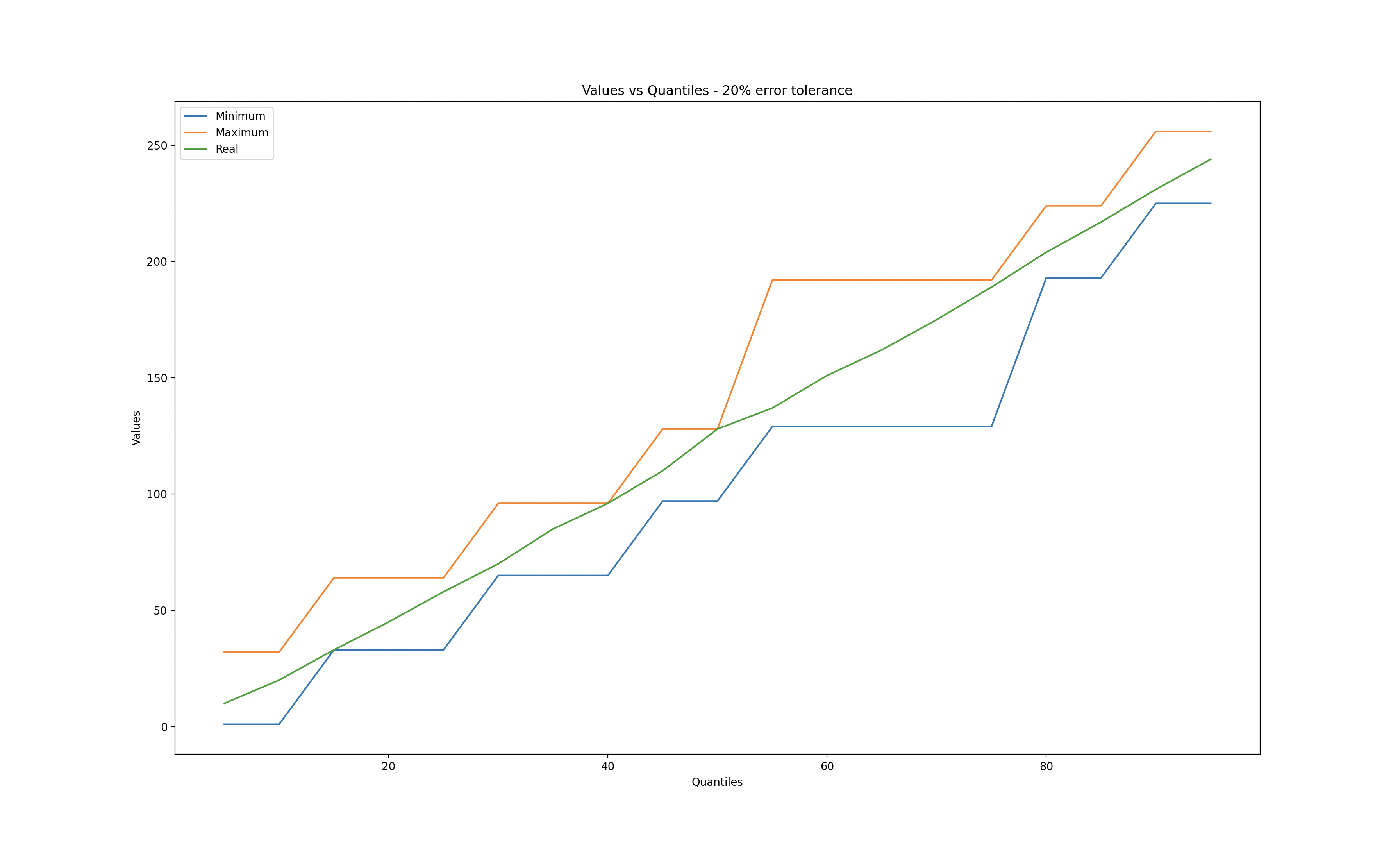
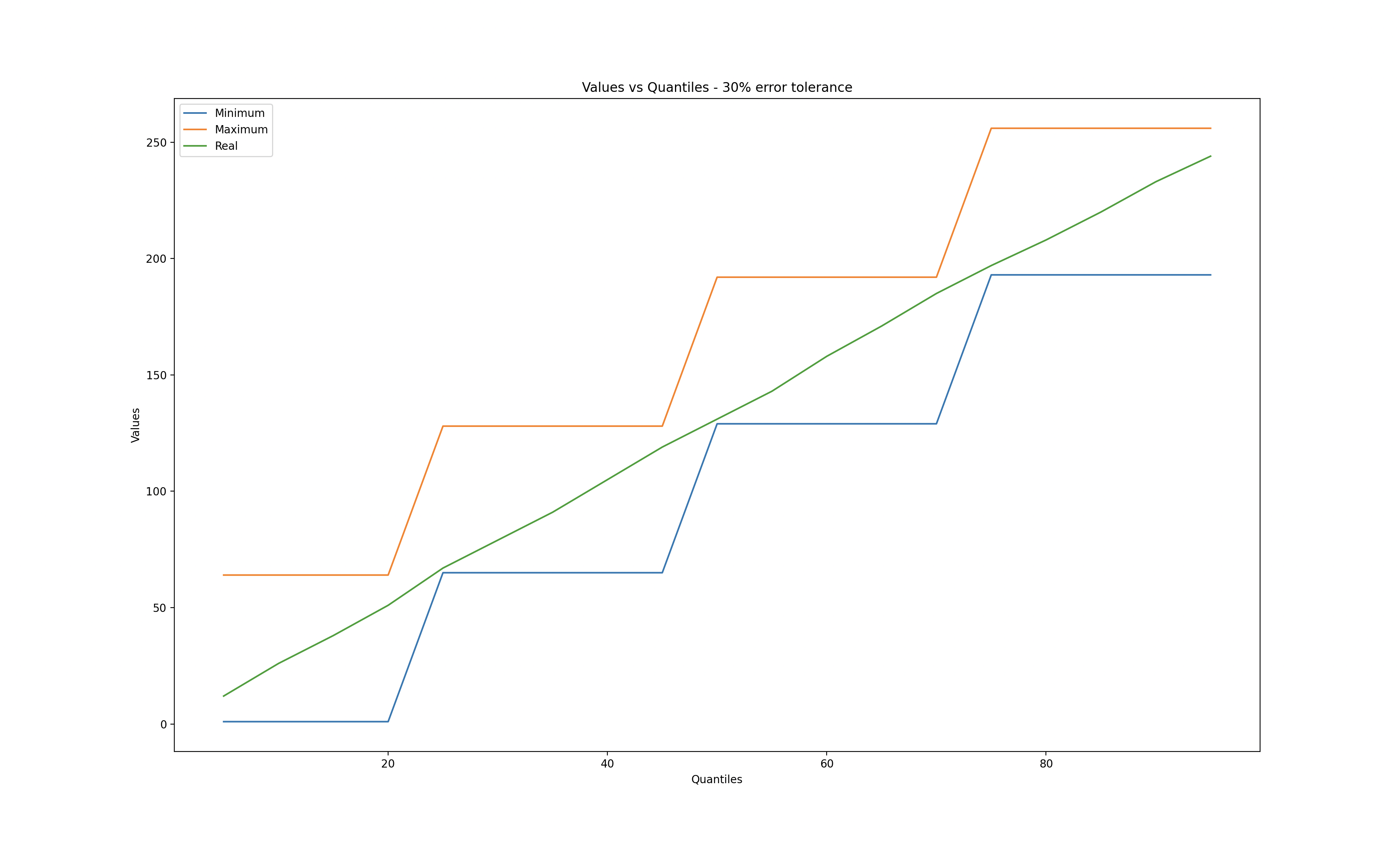
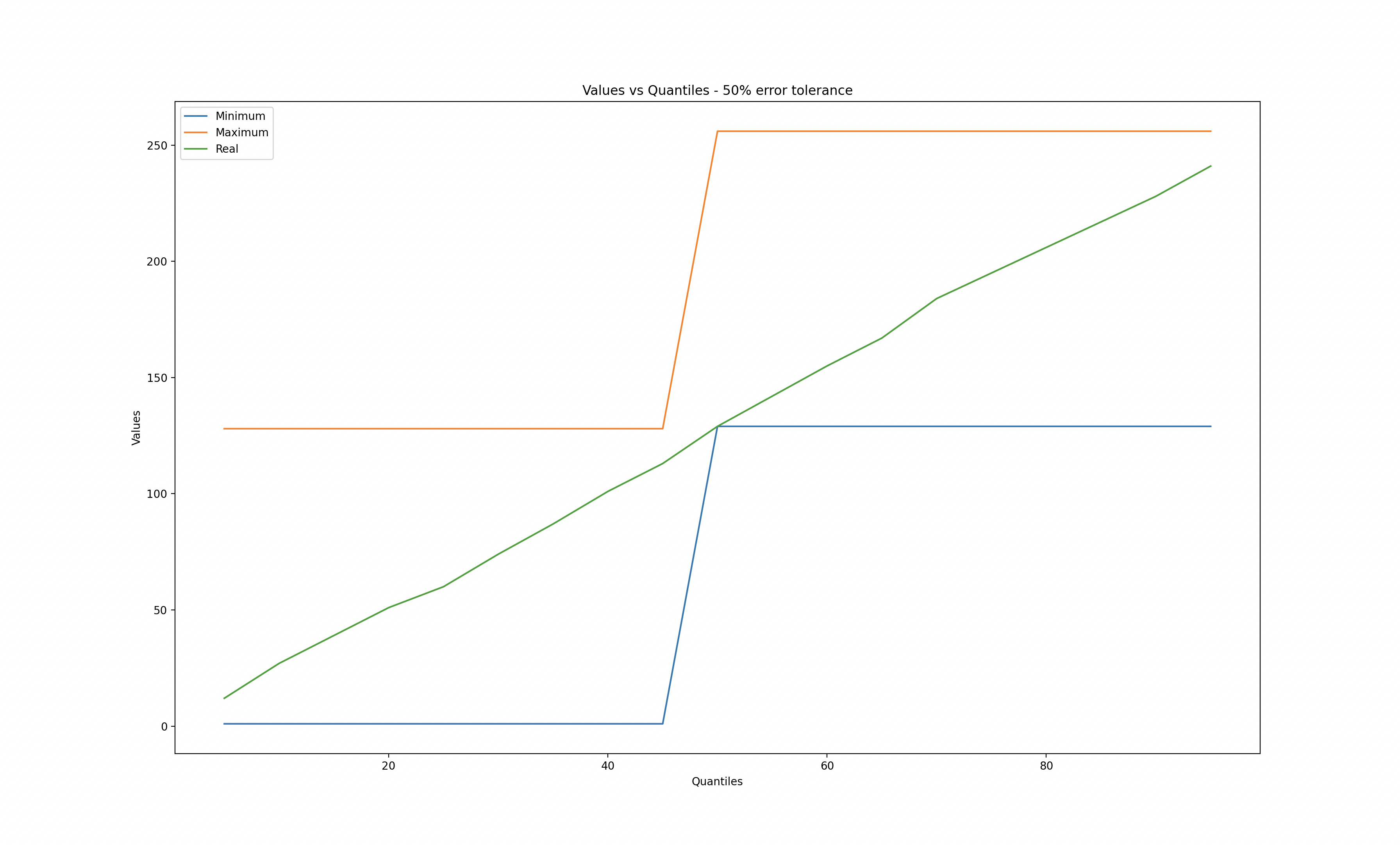
I used matplotlib to explore different error tolerances while calculating quantiles.
When the error tolerance is zero, we observe that the q-digest values match the real values. Conversely, when the error tolerance reaches 50%, a significant deviation is evident.
Zero error tolerance
10% error tolerance
20% error tolerance
30% error tolerance
50% error tolerance
References
Medians and Beyond: New Aggregation Techniques for Sensor Networks
Probabilistic Data Structures and Algorithms for Big Data Applications
1 In quest this is handled gracefully, if inputs exceed the bounds of the q-digest then they default to said bounds. Eg, if the q-digest for the age dataset gets an input of 0, this will be recorded as 1 as this is the minimum and if it gets another input of 512 this will be recorded as 8 as this is the maximum.